My Own Whole-Genome Sequencing Report
Beyond the usual disease and drug-response variants, a genome can tell you where your ancestors came from, how much archaic human DNA you carry, your blood-group and immune lineages, copy numbers and polygenic risk.
Contents
I have spent years analysing other people's sequencing data, and I got curious about what my own genome could tell me. I browsed the consumer genetic tests on Taobao and found most of them poor value. In the end I contacted a sequencing company I used to send samples to, paid CNY 1,600 (about US$220), and mailed them one purple-top tube of blood. About a month later they sent me a download link for the raw data: 88.8 Gb (about 88.8 billion bases), packed into two compressed files totaling 36.8 GB. Since I could analyse it myself, I took the chance to put what I know in order. This post first explains how whole-genome sequencing (WGS) works, then uses AI to run every analysis WGS allows, which I packaged into a skill.
1. How sequencing works#
Blood for DNA sequencing is usually collected in an EDTA tube (purple cap); 2–5 ml is plenty. Painless cheek-swab kits exist, but DNA from blood is of higher quality, so I sent a tube of blood. Sequencing itself has three steps: turn the DNA into a "library", run it on the sequencer, and translate millions of images into bases.
From blood to a "library"#
Only white blood cells have nuclei, so the DNA comes from them. A sequencer can read only one or two hundred bases at a time, so the DNA is first broken into fragments, "adapters" are ligated to both ends, and the result is a "library" of several hundred million short pieces:
Animation: library preparation — blood draw, DNA from white blood cells, sonication, adapter ligation, size selection and PCR, then 150 bases read from each end.
According to the company's report, my library was made exactly this way: sonication, end repair, A-tailing, adapter ligation, size selection and PCR amplification. After alignment, the positions of each read pair tell us how long the original fragment was:
Fragment (insert) length of my read pairs: median 312 bp, mean 320.8 bp (SD 70.6); 37% of fragments are shorter than 300 bp, so their two 150-base reads overlap.
The median fragment length is 312 bp. With 150 bases read from each end, most fragments leave only a short stretch in the middle unread; about 37% of fragments are shorter than 300 bp, so their two reads overlap.
How the sequencer "reads" DNA: sequencing by synthesis#
Illumina sequencers use "sequencing by synthesis"1. The library is spread over a chip called a flow cell, which carries billions of regularly arranged nanowells2. The fragment in each well is amplified in place into a few thousand identical copies (a "cluster") so the fluorescence is bright enough. Then, cycle after cycle: add fluorescent nucleotides whose ends are "blocked" → each strand takes exactly one → take a picture → cleave off the dye and the block, and start the next cycle. Each cycle reads one base of every cluster.
Animation: sequencing by synthesis — each cycle adds fluorescent, 3′-blocked nucleotides, one base joins each strand, a blue and a green image are taken (A blue only, T green only, C both, G neither), then dye and block are cleaved. Identical reads in neighbouring wells are optical duplicates.
To image faster, the NovaSeq X series uses only two dyes, blue and green: blue only is A, green only is T, both is C, and neither is G3.
My data did come from NovaSeq X instruments: the instrument IDs in the read names, LH00190, LH00750 and LH00281, all start with LH. The 592 million reads come from 3 lanes on 3 sequencers, 79% from one of them. Each lane mixes libraries from many people, separated by the "barcodes" in the adapters.
How accurate: quality scores#
Every base carries a quality score Q that expresses the chance it is wrong: Q = −10 × log₁₀(error probability)4. Q20 means 1 in 100, Q30 1 in 1,000, Q40 1 in 10,000. The NovaSeq X outputs only four quality levels (Q2, Q9, Q24, Q41), and 97.5% of my bases are at the top level, Q41. The chart shows, for each sequencing cycle, how many bases are not at the top level:
Per-cycle base quality (NovaSeq X, 4 quality levels Q2/Q9/Q24/Q41): 97.51% of bases are Q30 or better; even in the worst cycle 95.9% of bases are at the top level Q41. Quality declines slowly towards the end of each read.
Quality slowly declines towards the end of the reads, and the first few cycles are slightly worse too; but even in the worst cycle about 96% of bases are top quality.
Enough reads? Why read everything 20-odd times#
88.8 Gb divided by a genome of about 3.1 billion bases means each position is read about 29 times on average. But reads land on the genome at random: some positions get many, some few. If a position is read only three or four times, all the reads may come from the same copy, and a heterozygous variant is missed.
Interactive simulation: the higher the mean depth, the lower the chance of missing a heterozygous site (simplified rule: at least 3 reads for each base); beyond 30× the gain is small.
My real data:
Depth of coverage across the autosomes (gaps in the reference excluded): mean 21.56×; the distribution is wider than an ideal Poisson. X chromosome 10.7× (one copy in a man).
| Read at least | Share of autosomal positions |
|---|---|
| 1× | 99.7% |
| 5× | 99.2% |
| 10× | 98.3% |
| 15× | 90.5% |
| 20× | 62.4% |
| 30× | 7.6% |
After removing duplicate reads, the mean autosomal depth is 21.6× (the roughly 4.6% of the reference that is still unresolved gaps is excluded); 98.3% of positions are read at least 10 times and 62% at least 20 times5. The real distribution is wider than an ideal Poisson, because regions with very high or low GC content or many repeats are hard to sequence and hard to align.
Two interesting numbers: the X chromosome has a depth of only 10.7×, because men have a single X, which is also how sex is inferred from the data; mitochondrial DNA reaches 1,028×, because each cell holds close to a hundred copies of it.
Most of the drop from 29× to 21.6× is because 27% of read pairs are duplicates6: the same DNA molecule was read more than once. 21.8% are "optical duplicates", where one molecule spilled into a neighbouring well on the chip (the last step of the animation above shows this); 5.5% come from PCR. Duplicates add no information, so only one read per group is kept. Separately, contamination with someone else's DNA is estimated at just 0.06%7.
2. What the data look like: FASTQ, BAM, VCF#
The company delivered two gzip files, 36.8 GB together. They hold all the short fragments (FASTQ). Using the reference genome we assemble these fragments into my own genome (BAM), and then work out where my genome differs from the reference (VCF). Below I use a common variant in the TTN gene on chromosome 2 as the example. TTN encodes titin, the largest protein in the human body.
FASTQ: raw reads#
FASTQ is what the sequencer writes directly8: four lines per read, namely a name, the bases, a plus sign, and the quality of each base. My two files hold the first and second ends of the read pairs, 296 million each. Here is one of them:
One read from the raw FASTQ (4 lines: name, bases, +, qualities):
@LH00190:1151:25522TLT4:7:1209:49365:24231 1:N:0:GAACTGCAGA+GTTCGGTTAG
CGGTGCTACATTGATGATCTTAAGGCCAGATACTTTGTTGAAGAAGCTTATTTTGTATTTGTTGTCACTTGTTAGCTCTTTTCCATCCTTAAACCACTTAGTACTGAGTTCAGGGGTGCCAGCTACTGTACACTCCAAGGTACAGGTGTC
+
JJJJJJJJJJJJ9JJJJJJJJJJJJJJJJJJJJJJJJJJJJJJJJJJJJJJJJJJJJJJJJJJJJJJJJJJJJJJJJJJJJJJJJJJJJJJJJJJJJJJJJJJJJJJJJJJJJJJJJJJJJJJJJJ9JJJJJJJJJJJJJJJJJJJJJJJ
BAM: reads placed back on the reference#
The reference genome goes back to the Human Genome Project and has been through many versions since. It does not belong to any one person; it is assembled from the DNA of a handful of people, and works like a dictionary. Once my fragments are aligned to it, every read gets an "address": which chromosome, which base, which strand, and how well it fits. This is stored in a BAM file9, sorted by position and indexed, so any region can be pulled up like a map. My BAM is 29.7 GB, and the CRAM format would compress it further10. Stacking all reads that cover the same position gives a "pileup":
Pileup of 29 reads at a common synonymous SNP in TTN (chr2:178,714,003, rs2562839): 10 reads show the reference G and 10 show A, about half each, so the site is heterozygous.
VCF: the final list of differences#
What actually needs interpreting is only "where I differ from the reference". Variant calling picks these out and writes them into a VCF file11: one site per line, position and bases first, my genotype and the supporting evidence in the last column.
The VCF line for this site (DeepVariant output):
#CHROM POS ID REF ALT QUAL FILTER INFO FORMAT zhh
chr2 178714003 . G A 43.5 PASS . GT:GQ:DP:AD:VAF:MID:PL 0/1:43:20:10,10:0.5:small_model:43,0,59
My VCF holds about 4.97 million variants:
Differing from the reference at millions of positions is completely normal: the reference itself is stitched together from only a few people's DNA12, and whether any difference matters clinically needs further interpretation.
From 37 GB to 0.1 GB#
File size at each step:
| File | Size |
|---|---|
| FASTQ (two compressed files) | 36.8 GB |
| BAM (aligned) | 29.7 GB |
| gVCF (incl. non-variant blocks) | 1.5 GB |
| VCF (variants only) | 106 MB |
A BAM is about as large as the FASTQ: no read is dropped, they only gain positions. The VCF is down to about 0.1 GB, more than 300 times smaller than the raw data. A gVCF also records "which positions are confirmed to match the reference", which you need when analysing your data jointly with other people's. I keep the raw data in cloud storage, and it is worth keeping for good: with better variant callers or a newer reference, everything can be re-analysed from scratch.
3. How WGS analysis works#
The whole pipeline ran on my own workstation: alignment took 27.5 minutes and variant calling 27 minutes, using an RTX 4090 graphics card (so coveted in China that it is nicknamed "electronic Moutai", after the famously expensive liquor) and NVIDIA's GPU-accelerated tools13.
Alignment: finding a place for 590 million reads#
The reference genome is GRCh3812. The aligner, BWA-MEM14,15, works by "look up the index first, then align in detail":
Animation: how BWA-MEM aligns a read — exact-match seeds are looked up in the reference's FM index, candidate positions are extended and scored base by base, and the best score wins.
After alignment, duplicates are marked and reads are sorted by position, which gives the BAM from the previous chapter. 99.82% of my reads align; the remaining 0.18% (1.07 million) find no place on the human reference, and most of them are not human DNA. If there is a virus in the blood, its reads end up in this pile, which is why chapter 6 searches these 1.07 million reads for viruses.
Variant calling: looking at the pileup as an image#
Classic variant callers use statistical models: count how many reads at each position support the reference base and how many support another, and factor in the quality scores. DeepVariant16 takes another route: it draws the pileup as a multi-channel "image" and lets a convolutional neural network, the kind designed to recognise photos, decide the genotype.
Animation: DeepVariant draws the pileup as a multi-channel image (base, base quality, mapping quality, strand, supports variant, differs from reference) and a convolutional neural network outputs the probabilities of the three genotypes.
When several people are analysed together, GLnexus17 merges everyone's gVCF so all of them are judged by the same standard at the same position.
Annotation: what does this variant do#
A VCF only has positions and bases. Knowing what a variant "does" requires annotation18: which gene it is in, whether it changes an amino acid, how common it is in the population (gnomAD19), whether it has been reported as pathogenic (ClinVar20), and scores from various predictors: REVEL21 and AlphaMissense22 for missense variants, SpliceAI23 for splicing.
The example above annotates as: TTN c.26655C>T, position 8885 stays serine (a synonymous variant); in gnomAD 31% of chromosomes carry the A, 65% among East Asians. Very common and protein-neutral, so it can be treated as a harmless common variant.
Picking the few worth a look out of millions#
Filtering all variants down to the few that need a human look:
| Step | Variants |
|---|---|
| All variants | 4,970,671 |
| Near exons (±50 bp) | 369,448 |
| May change protein or splicing | 19,667 |
| Of these, population frequency < 1% | 690 |
| Predicted damaging or listed as pathogenic; needs manual review | 49 |
| Confirmed pathogenic in the 84 ACMG actionable genes | 0 |
The vast majority of variants lie between genes or in introns. Fewer than 20,000 fall near exons and might change a protein or splicing; of these only 690 are rare in the population (frequency below 1%); filtering by functional predictions and ClinVar leaves 49 that need a human to look at. After checking each one against read quality and the literature and classifying it by the ACMG/AMP criteria24: there is no pathogenic variant in the 84 actionable genes ACMG recommends reporting25, and the rest are mostly of uncertain significance or benign. Recessive carrier results are not covered here (see chapter 8).
What comes next#
| Chapter | Question | Principle | Main tools and data |
|---|---|---|---|
| 4. Where I come from | Which modern and ancient populations I resemble most, and which ancestral sources I am a mix of | Compare allele frequencies at hundreds of thousands of sites; close populations share more "genetic drift" | smartpca26, ADMIXTOOLS27, AADR28 |
| Does each chromosome segment look northern or southern | Separate the two copies (phasing), then compare segment by segment along each chromosome with reference populations | Beagle29, RFMix30 | |
| How much Neanderthal DNA do I carry | Find variants that are absent in Africans and occur in runs, then compare them with archaic genomes | hmmix31 | |
| Are my parents related | Look for long stretches where both copies are identical | bcftools roh32 | |
| Which paternal and maternal lineages | Place Y-chromosome and mitochondrial variants on the phylogenetic tree | Yleaf33, HaploGrep 334 | |
| 5. Biological age | Signs of ageing in blood DNA | Depth ratios, low-fraction somatic mutations, counting telomere repeats | TelSeq35 |
| 6. Immunity and blood | Blood groups, HLA and KIR, viruses | Convert key sites into antigens; compare reads with known alleles; classify non-human reads by sequence | T1K36, Kraken237 |
| 7. Copy number | Which genes have an extra or a missing copy | Depth of a region relative to the genome-wide mean | My own scripts |
| 8. Medically relevant findings | Pathogenic variants and drug response | The filtering above, plus pharmacogenomic guidelines | PharmCAT38, CPIC39 |
| 9. Polygenic risk | Is my "genetic background" for a disease high | Weighted sum of hundreds to thousands of small-effect variants, compared with people of the same ancestry | PGS Catalog40, PLINK 241 |
| 10. Repeat expansions | Any pathogenic repeat expansion | Count the repeat units in reads that span the repeat | ExpansionHunter42 |
4. Where I come from#
Where I stand on the genetic map of East Asia#
Ancient-DNA databases collect genomes of people who lived long ago, and they are the best reference for tracing one's own origins. Compress the genomes of dozens of modern East Asian populations into two coordinates: the horizontal axis runs roughly north to south, and the vertical axis pulls the Japanese archipelago apart. I fall between Northern Han Chinese (Beijing) and Southern Han Chinese, closer to the southern side, very near the HGDP43 Han samples and the Tujia.
Switching to "Ancient individuals" is more interesting: with more than three thousand ancient people projected into the same space, I stand right between Late Neolithic to Shang–Zhou populations of the middle and lower Yellow River and Neolithic to Iron Age populations of Fujian, Penghu and Taiwan.
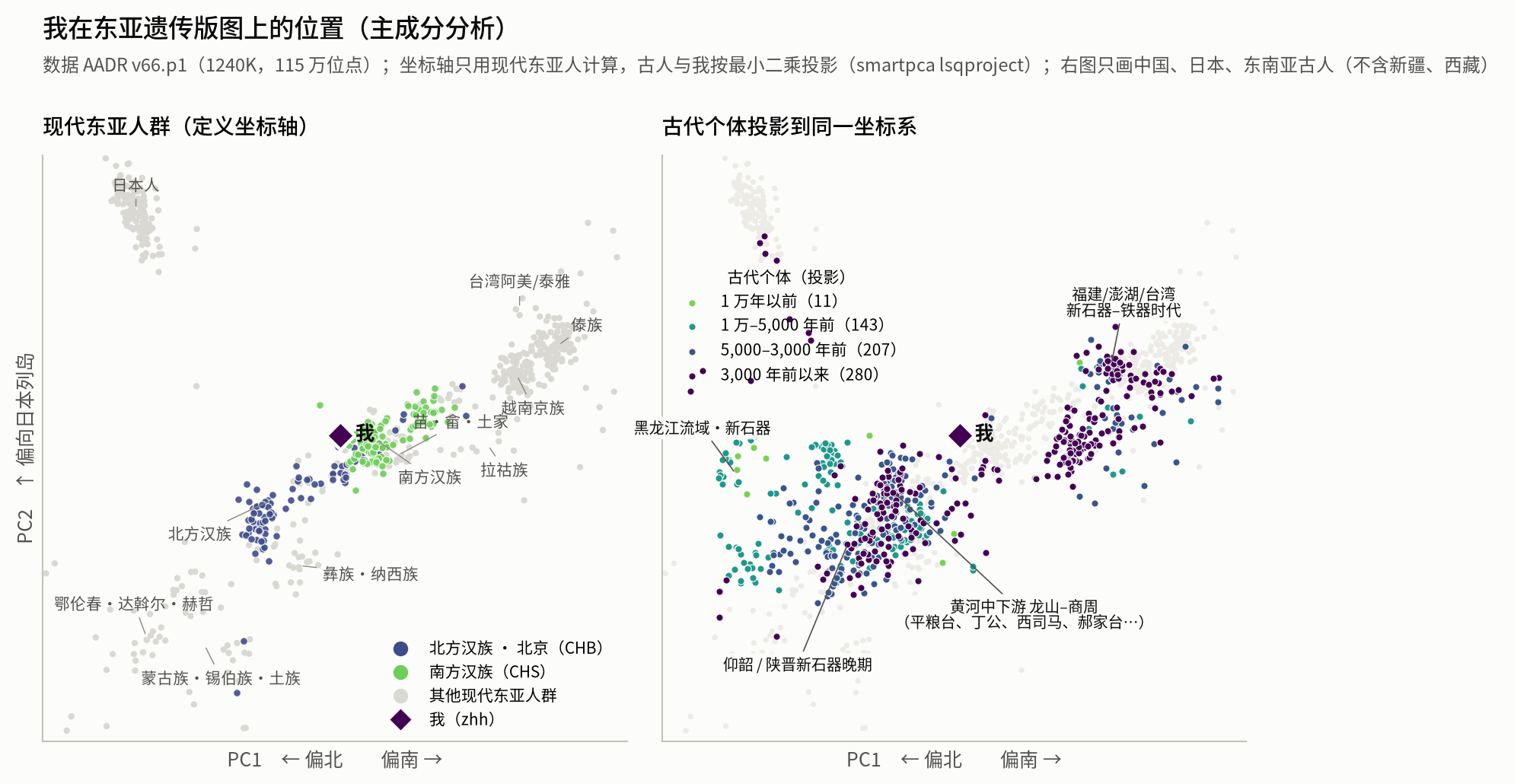
Principal component analysis of modern East Asians (PC1 runs roughly north to south, PC2 separates the Japanese archipelago), with ancient individuals and me projected. Closest modern populations to me: Han (HGDP); Southern Han (1000G); Tujia; She; Miao. Closest ancient groups (≥ 3 individuals): Dasongshan, Guizhou · Ming dynasty; Baligang, Henan · Longshan culture; Baligang, Henan · Shijiahe culture; Weifang, Shandong · Zhou dynasty; Dinggong, Shandong · Longshan culture; Baligang, Henan · Eastern Zhou.
Method: the 1240K sites of the ancient-DNA dataset AADR v66.p128 (June 2026), 1.15 million SNPs in total; my genotypes at these sites were read directly from the whole-genome data (coordinates lifted from hg19 to hg38, 99.8% called). smartpca26 computed the axes from modern East Asians only; ancient individuals and I were projected by least squares. Modern populations are from 1000 Genomes44,45 and HGDP.
Compared with ancient people: whom do I resemble most#
For more than 500 ancient populations in and around East Asia I computed a score for "how much genetic history they share with me" (outgroup f3; higher means more similar). Darker colours mean more similar. You can switch between time periods, and drag the colour bar below to show only a range of scores.
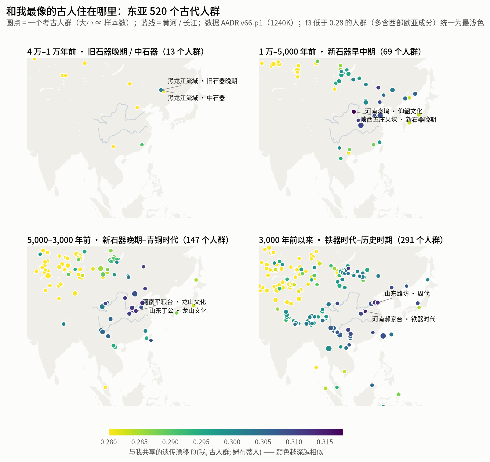
Map of outgroup f3(me, ancient population; Mbuti) for 543 ancient populations in and around East Asia (higher = more shared genetic history). The ten highest: Wuzhuangguoliang, Shaanxi · Late Neolithic (0.3180); Haojiatai, Henan · Iron Age (0.3135); Dinggong, Shandong · Longshan culture (0.3130); Weifang, Shandong · Zhou dynasty (0.3128); Pingliangtai, Henan · Longshan culture (0.3125); Tonglin, Zibo, Shandong · Eastern Zhou (0.3124); Selenge, Mongolia · Xiongnu period (0.3119); Xisima, Henan · Late Shang (0.3117); Xiaowu, Henan · Yangshao culture (0.3117); Wadian, Henan · Longshan culture (0.3117).
Whatever the period, the points most similar to me (the darkest) are always on the middle and lower Yellow River: Neolithic Xiaowu in Henan (Yangshao culture) and Wuzhuangguoliang in Shaanxi, Longshan-culture Pingliangtai in Henan and Dinggong in Shandong46–48, and on to Shang–Zhou populations of Henan and Shandong.
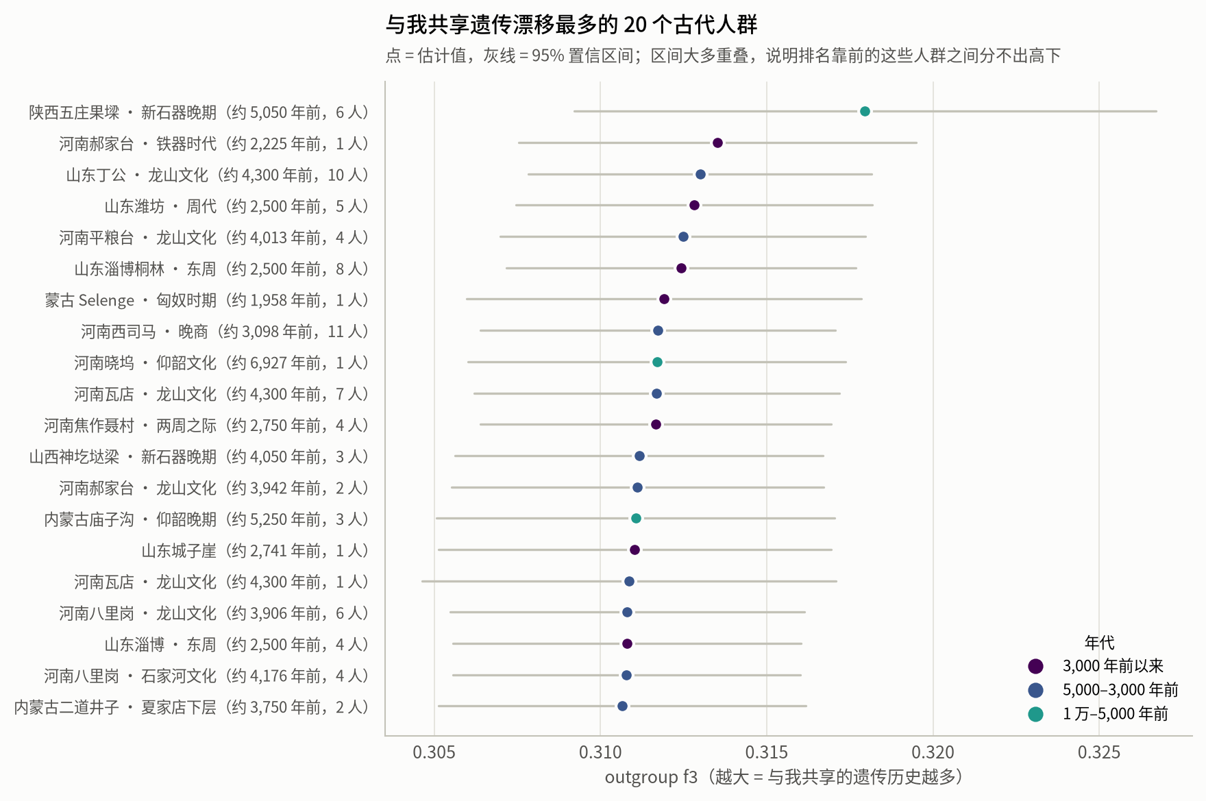
The 20 ancient populations sharing the most genetic drift with me (outgroup f3; the 95% confidence intervals overlap heavily):
| Rank | Population/site | Age | N | f3 | 95% CI |
|---|---|---|---|---|---|
| 1 | Wuzhuangguoliang, Shaanxi · Late Neolithic | c. 5,050 years ago | 6 | 0.3180 | 0.3092–0.3267 |
| 2 | Haojiatai, Henan · Iron Age | c. 2,225 years ago | 1 | 0.3135 | 0.3075–0.3195 |
| 3 | Dinggong, Shandong · Longshan culture | c. 4,300 years ago | 10 | 0.3130 | 0.3078–0.3182 |
| 4 | Weifang, Shandong · Zhou dynasty | c. 2,500 years ago | 5 | 0.3128 | 0.3075–0.3182 |
| 5 | Pingliangtai, Henan · Longshan culture | c. 4,013 years ago | 4 | 0.3125 | 0.3070–0.3180 |
| 6 | Tonglin, Zibo, Shandong · Eastern Zhou | c. 2,500 years ago | 8 | 0.3124 | 0.3072–0.3177 |
| 7 | Selenge, Mongolia · Xiongnu period | c. 1,958 years ago | 1 | 0.3119 | 0.3060–0.3178 |
| 8 | Xisima, Henan · Late Shang | c. 3,098 years ago | 11 | 0.3117 | 0.3064–0.3171 |
| 9 | Xiaowu, Henan · Yangshao culture | c. 6,927 years ago | 1 | 0.3117 | 0.3060–0.3174 |
| 10 | Wadian, Henan · Longshan culture | c. 4,300 years ago | 7 | 0.3117 | 0.3062–0.3172 |
| 11 | Niecun, Jiaozuo, Henan · Western–Eastern Zhou transition | c. 2,750 years ago | 4 | 0.3117 | 0.3064–0.3169 |
| 12 | Shengedaliang, Shanxi · Late Neolithic | c. 4,050 years ago | 3 | 0.3112 | 0.3056–0.3167 |
| 13 | Haojiatai, Henan · Longshan culture | c. 3,941 years ago | 2 | 0.3111 | 0.3055–0.3167 |
| 14 | Miaozigou, Inner Mongolia · Late Yangshao | c. 5,250 years ago | 3 | 0.3111 | 0.3051–0.3170 |
| 15 | Chengziya, Shandong | c. 2,741 years ago | 1 | 0.3110 | 0.3051–0.3169 |
| 16 | Wadian, Henan · Longshan culture | c. 4,300 years ago | 1 | 0.3109 | 0.3046–0.3171 |
| 17 | Baligang, Henan · Longshan culture | c. 3,905 years ago | 6 | 0.3108 | 0.3055–0.3161 |
| 18 | Zibo, Shandong · Eastern Zhou | c. 2,500 years ago | 4 | 0.3108 | 0.3056–0.3160 |
| 19 | Baligang, Henan · Shijiahe culture | c. 4,176 years ago | 4 | 0.3108 | 0.3056–0.3160 |
| 20 | Baligang, Henan · Qujialing culture | c. 4,582 years ago | 2 | 0.3107 | 0.3049–0.3164 |
Almost all of the top 20 come from Henan, Shandong, Shaanxi and Shanxi, plus a Late Yangshao site in Inner Mongolia (Miaozigou) and a Lower Xiajiadian site (Erdaojingzi)46. Their confidence intervals overlap heavily, though: these populations are very similar to one another, so statistically none of them is "the" closest to me. Taken together, my main ancestry continues from the populations of the Yellow River basin since the Neolithic.
Interestingly, the ranking includes a person buried in a Xiongnu-period cemetery in Selenge Province, Mongolia (directly dated to 52 BCE–62 CE)49, whose similarity to me is on a par with the ancient people of the Central Plains. The Xiongnu were a genetically very diverse steppe confederation that included members genetically close to Central Plains populations.
Method: ADMIXTOOLS27 qp3Pop computing f3(me, ancient population; Mbuti); only populations covering ≥ 30,000 sites are shown. The map shows only coastlines and the Yellow and Yangtze rivers, without national borders.
Splitting my genome into "northern + southern" sources#
qpAdm is the standard ancient-DNA method for testing whether a population can be modelled as a mix of several sources, and in what proportions50,51. I modelled two sources: Longshan-era farmers of the middle Yellow River (Pingliangtai, Haojiatai and Wadian in Henan, Shengedaliang in Shanxi, and others)46,48, and southern coastal populations (Late Neolithic Tanshishan and Xitou in Fujian and Penghu52, or Iron Age Hanben in Taiwan47).
qpAdm two-source models: my genome = northern source (Late Neolithic Yellow River) + southern source; p ≥ 0.05 means two sources fit.
| Model | Outgroups | Northern | Southern | SE | p |
|---|---|---|---|---|---|
| Yellow River Longshan + Fujian/Penghu Neolithic | base outgroups | 74.9% | 25.1% | 10.3% | 0.14 |
| Yellow River Longshan + Fujian/Penghu Neolithic | extended outgroups | 92.4% | 7.6% | 5.1% | 0.12 |
| Yellow River Longshan + Taiwan Hanben | base outgroups | 70.2% | 29.8% | 9.7% | 0.29 |
| Yellow River Longshan + Taiwan Hanben | extended outgroups | 86.2% | 13.8% | 6.2% | 0.18 |
| Shandong Longshan + Fujian/Penghu Neolithic | base outgroups | 56.7% | 43.3% | 9.3% | 0.0048 |
| Shandong Longshan + Fujian/Penghu Neolithic | extended outgroups | 85.4% | 14.6% | 4.8% | 0.0000012 |
| Shandong Longshan + Taiwan Hanben | base outgroups | 55.1% | 44.9% | 7.7% | 0.067 |
| Shandong Longshan + Taiwan Hanben | extended outgroups | 75.1% | 24.9% | 5.5% | 0.000058 |
| Yellow River Yangshao + Taiwan Hanben | base outgroups | 75.3% | 24.7% | 12.2% | 0.14 |
| Yellow River Yangshao + Taiwan Hanben | extended outgroups | 81.4% | 18.6% | 6.2% | 0.16 |
With several combinations of sources, the two-source model explains my genome (p ≥ 0.05), with the northern component between about 70% and 90% depending on the choice of outgroups; a single Yellow River source is not enough (rejected).
Switch to "Me vs individual Han" to compare with the same model (Yellow River Longshan + Taiwan Hanben, base outgroups): six Beijing Han individuals have 86–100% northern ancestry, six Southern Han 42–75%, six HGDP Han 39–70%, and I am 70%, right between Northern and Southern Han, consistent with the PCA. One more detail: for most Beijing Han individuals two sources are enough, while most Southern Han individuals are rejected, meaning they carry ancestry from outside these two sources (such as populations further southwest).
This matches published work on modern Han Chinese: their ancestry is mainly from Neolithic Yellow River farmers, mixed with varying amounts of southern ancestry that increases further south47,52.
Method: ADMIXTOOLS 8 qpAdm (allsnps). Base outgroups: Mbuti, Ust'-Ishim, Kostenki 14, Papuan, Onge, Tianyuan, Ganj Dareh, Japanese Jōmon, Amur River Neolithic and Mongolia Neolithic47,53–61; the extended set adds Early Neolithic individuals from Shandong, Fujian and Guangxi52,62. In the other source combinations, the Shandong Longshan population comes from Dinggong, Chengziya and Yinjiacheng48,63. The "individual Han" panel uses 6 random people each from Beijing Han, Southern Han and HGDP Han; a single person as the target has about the same statistical power as me.
Chromosome painting: which segments look northern, which southern#
qpAdm gives a genome-wide average. If the two copies of each chromosome are separated (phased), and Beijing Han stand in for "northern East Asia" while Dai from Xishuangbanna and Kinh from Vietnam stand in for "southern East Asia", every segment of every chromosome can be "painted". Hold Ctrl and scroll, or drag the slider at the bottom, to zoom into a region; hover to see the position of each segment.
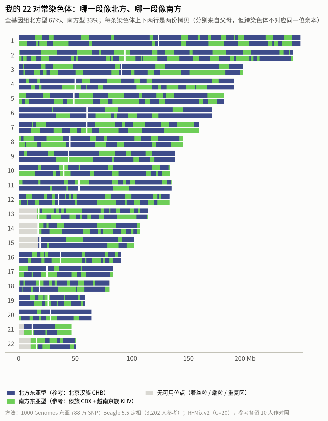
Chromosome painting (local ancestry, RFMix): each of the two copies of each autosome is painted northern East Asian (like Beijing Han) or southern East Asian (like Dai/Kinh). Genome-wide: 67% northern, 33% southern.
| Chromosome | Northern fraction |
|---|---|
| 1 | 73% |
| 2 | 62% |
| 3 | 66% |
| 4 | 71% |
| 5 | 56% |
| 6 | 81% |
| 7 | 51% |
| 8 | 61% |
| 9 | 73% |
| 10 | 73% |
| 11 | 79% |
| 12 | 69% |
| 13 | 51% |
| 14 | 59% |
| 15 | 78% |
| 16 | 65% |
| 17 | 73% |
| 18 | 68% |
| 19 | 67% |
| 20 | 80% |
| 21 | 55% |
| 22 | 50% |
The two rows of each chromosome are its two copies (one from my father, one from my mother; which parent is not matched across chromosomes). Overall about 67% is northern and 33% southern, and the fine interleaving of the two colours shows that thousands of years of intermarriage have cut my ancestors' DNA into very short pieces.
To check how far this reading can be trusted, I scored 1000 Genomes individuals who were left out of the reference panel in the same way (10 per group):
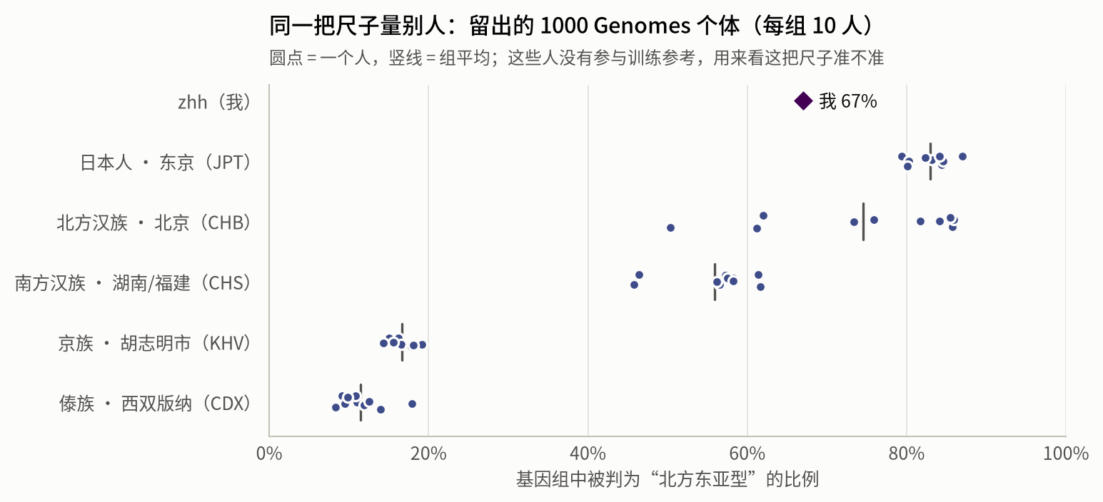
The same method applied to held-out 1000 Genomes individuals (10 per group):
| Population | Northern fraction (median) |
|---|---|
| Northern Han (Beijing) | 79% |
| Japanese | 84% |
| Southern Han | 57% |
| Kinh (Vietnam) | 16% |
| Dai (Xishuangbanna) | 11% |
| Me | 67% |
The medians are 79% for Beijing Han, 84% for Japanese, 57% for Southern Han, 16% for Kinh and 11% for Dai. I am at 67%, between Beijing Han and Southern Han, consistent with the PCA and qpAdm. Populations within East Asia differ very little, so the call for any single short segment has a sizeable error, but the overall proportion is more reliable.
Method: my genotypes at 7.88 million SNPs with frequency ≥ 1% in 1000 Genomes East Asians; phasing with Beagle 5.529 using the phased haplotypes of 3,202 1000 Genomes individuals45 as reference; local ancestry with RFMix v230 (G = 20 generations of admixture), with about 90 Beijing Han and about 170 Dai and Kinh as references, plus 10 of each held out as controls.
Paternal and maternal lines#
- Paternal (Y chromosome): O-M175 › O-M122 › O-M134 › O-Y20 › O-F79 › O-CTS10739 › O-MF1484 (YFull tree64), which the FTDNA tree65 subdivides further to O-PH233. O-M134 is one of the most common paternal branches among Han Chinese. YFull estimates that O-MF1484 split from its sister branch about 7,400 years ago; the other samples under it in the database come from Jiangsu and Beijing.
- "Kin" in ancient DNA: two ancient individuals in the AADR belong to my upstream branch O-Y20: a Yangshao-culture man from Baligang, Dengzhou, Henan, about 6,000 years ago66, and an Iron Age individual from Yunnan about 2,300 years ago67. O-Y20 itself is thousands of years old, so sharing it does not imply a close relationship.
- Maternal (mitochondria): B4c1b2c. Its sub-branch B4c1b2c2 was found in an individual from the Lajia site in Qinghai about 3,900 years ago (Qijia culture)46. She and I belong to the same branch, B4c1b2c; one level up, B4c1b2 also appears among 7th-century Avars in Hungary68,69, a group that migrated from the East Asian steppe to Europe.
Method: Yleaf v4.1.533 with three trees, YFull v14.01, FTDNA and ISOGG70 (consistent results, quality score 1.0); mitochondria with HaploGrep 334. Haplogroups of ancient individuals are from the AADR annotation table.
The Neanderthal and Denisovan in me#
Going further back in time, every modern human whose ancestors left Africa carries traces of interbreeding with Neanderthals and Denisovans tens of thousands of years ago. I found 1,051 segments of archaic origin, about 104 Mb in total; among those whose source can be assigned, about 80 Mb are Neanderthal-like and about 5.5 Mb Denisovan-like (about 0.1% of the genome, in line with published values for East Asians71). Among the Neanderthal segments, more are closest to the Vindija Neanderthal from Croatia (270) than to either of the two Neanderthals from the Altai Mountains in Siberia (Altai and Chagyrskaya, about 210 each). This too agrees with the known finding that the Neanderthals who interbred with modern humans were closer to Vindija72. That is why I have always thought of our genes not as a snapshot of the present, but as an ancient book handed down over tens of thousands of years, full of stories from long ago.
Hover to see each segment's position, length, the number of variants shared with four archaic genomes, and the genes it covers; you can also type a gene name in the box at the top right.
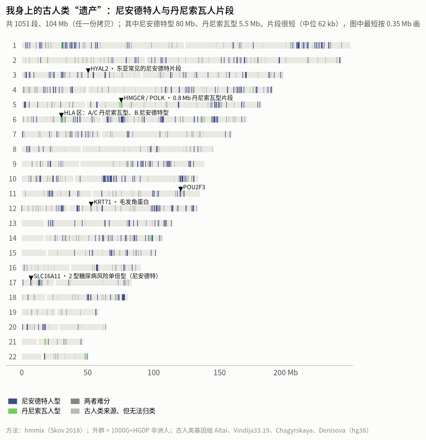
My archaic-human segments (hmmix): 1051 segments, 104 Mb in total; Neanderthal-like 80.4 Mb, Denisovan-like 5.5 Mb. Notable: SLC16A11 (type 2 diabetes risk haplotype, one copy), HLA region, HYAL2, POU2F3, KRT71, and a 0.8 Mb Denisovan-like segment near HMGCR/POLK on chromosome 5.
A few segments with a story:
- SLC16A11 (chromosome 17): a famous Neanderthal haplotype with a frequency of about 10% in East Asians; each copy raises the risk of type 2 diabetes by about 25%73. I am heterozygous at all 4 marker sites of this haplotype, so I carry one copy.
- The HLA region: the areas near HLA-A and HLA-C are called Denisovan-like, and near HLA-B Neanderthal-like. I happen to carry HLA-A*11:01, an HLA type common in East Asia that one study suggests came originally from Denisovans74. The HLA region is extremely polymorphic, so such calls are only hints.
- HYAL2, POU2F3: Neanderthal segments common in East Asians and thought to have possibly been under natural selection75,76; there is also one on the hair keratin gene KRT71, and keratin genes are a known hotspot of Neanderthal segments76,77.
- A 0.8 Mb Denisovan-like segment near HMGCR / POLK on chromosome 5 is my longest Denisovan-like segment; I found no study focused on this particular segment, so I note it only as a curiosity.
Is that a lot or a little? I took 8 people each of Northern Han, Southern Han, Japanese, Kinh and Dai from 1000 Genomes and re-ran exactly the same pipeline:
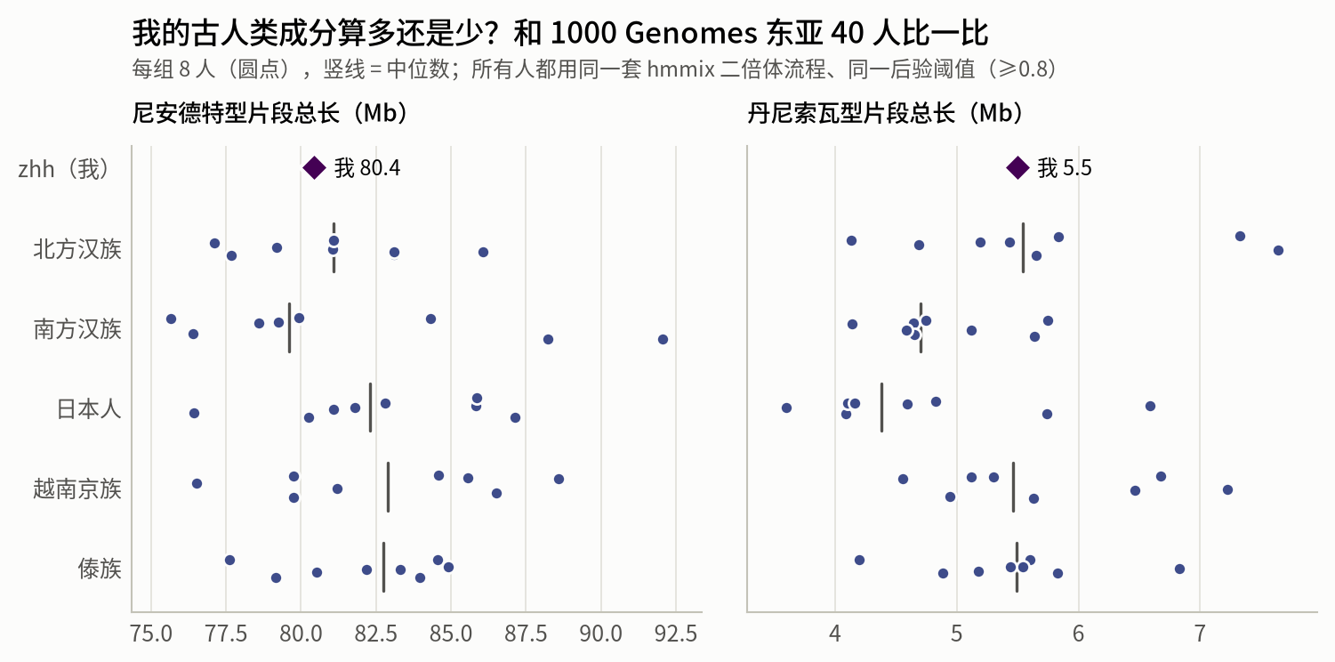
Archaic ancestry with the same pipeline, me vs 8 East Asians per 1000 Genomes group (medians):
| Population | Neanderthal-like Mb | Denisovan-like Mb |
|---|---|---|
| Northern Han (Beijing) | 81.1 | 5.5 |
| Southern Han | 79.6 | 4.7 |
| Japanese | 82.3 | 4.4 |
| Kinh (Vietnam) | 82.9 | 5.5 |
| Dai (Xishuangbanna) | 82.7 | 5.5 |
| Me | 80.4 | 5.5 |
My 80 Mb of Neanderthal-like DNA sits right in the middle, and so do my 5.5 Mb of Denisovan-like DNA: I am an East Asian in "standard configuration".
Method: hmmix31 diploid decoding with Africans from 1000 Genomes + HGDP as the outgroup; sources were assigned using 4 high-coverage archaic genomes (the Altai78, Vindija72 and Chagyrskaya79 Neanderthals and the Denisovan80), posterior probability ≥ 0.8. A segment sharing more derived variants with Neanderthals than with the Denisovan is called Neanderthal-like, and vice versa.
Are my parents related?#
If parents are close relatives, their child's genome contains long stretches where "both copies are identical" (runs of homozygosity, ROH).
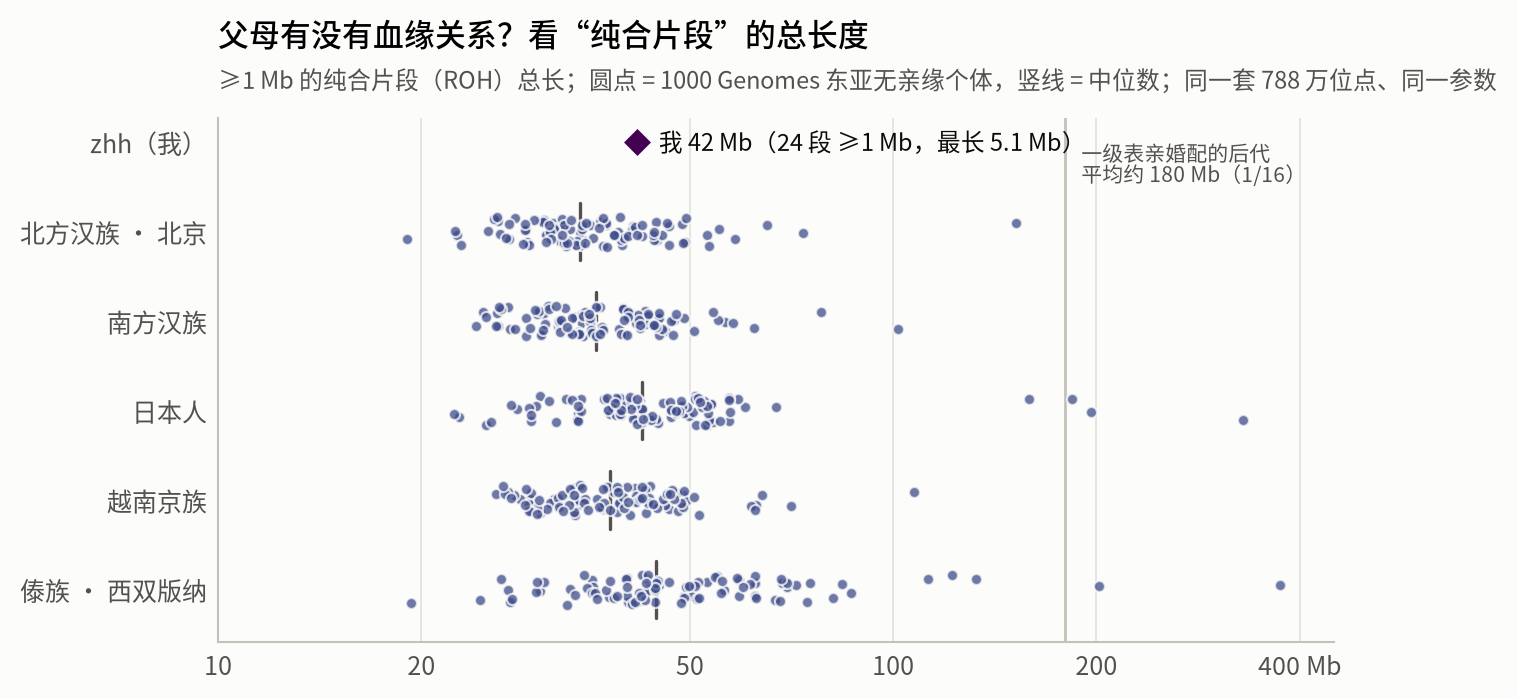
Runs of homozygosity ≥ 1 Mb: I have 24 runs, 42 Mb in total, the longest 5.1 Mb — in the normal East Asian range; the child of first cousins averages about 180 Mb.
| Population | Median total ROH Mb |
|---|---|
| Northern Han (Beijing) | 34 |
| Southern Han | 36 |
| Japanese | 42 |
| Kinh (Vietnam) | 38 |
| Dai (Xishuangbanna) | 44 |
I have 24 runs ≥ 1 Mb, 42 Mb in total, the longest 5.1 Mb, in the middle of the normal range for East Asians; the child of first cousins has about 180 Mb on average81. My parents are not closely related.
Method: bcftools roh32 with allele frequencies from 1000 Genomes East Asians and Beagle's GRCh38 genetic map; I and 506 East Asian controls used the same 7.88 million sites and the same parameters.
5. Molecular traces of age#
The DNA in my blood also holds a few signals related to ageing:
- Mitochondrial DNA copy number: about 96 copies per blood cell. It declines slowly with age and is also related to health82; absolute values differ greatly between methods, so it is only useful for comparing yourself with yourself.
- Clonal hematopoiesis (CHIP): with age, some blood stem cells acquire mutations in genes such as DNMT3A and TET2 and expand into clones, which is linked to blood cancers and cardiovascular risk83,84. I scanned the coding regions of 25 relevant genes; the only candidate (3 adjacent sites in IDH2) turned out on inspection to be an alignment artefact, supported by just 2 heavily clipped reads.
- Mosaic loss of Y: common in older men and linked to various diseases85; rare at my age anyway.
- Telomere length: estimated by counting TTAGGG repeats in the reads35. The absolute value depends heavily on library preparation and platform, so a single number means little; it is more useful to measure again with the same method in ten years and see how much mine has shortened.
6. Immune and blood typing#
Blood groups: more than ABO and Rh#
Hospitals test only ABO and RhD, but red cells carry more than 40 blood-group systems. A genome gives you a dozen or so of the common ones at once:
| System | My type | Common in East Asians? | Notes |
|---|---|---|---|
| ABO | Group A (A/O) | Common | Inferred from several sites; serology is definitive |
| Rh(D) | RhD positive (2 copies of RHD) | Over 99.5% of Han Chinese are positive | No "Asian-type DEL" variant either |
| Rh(E/e) | E+e+ | Common | C/c cannot be called reliably with short reads because RHD and RHCE are so similar |
| Duffy | Fy(a+b−) | About 90% | |
| Kidd | Jk(a+b+) | About 40–50% | |
| Kell | K−k+ | Almost everyone | The K antigen is very rare in East Asia |
| MNS | S−s+ | About 90% | M/N not typed (GYPA/GYPB are homologous) |
| Diego | Di(a−b+) | Over 90% | Di(a) occurs in about 3–10% of East Asians and is an uncommon cause of hemolytic disease of the newborn |
| Lewis / secretor | Le(a−b+), secretor | Common | FUT2 and FUT3 both normal |
| Dombrock / Colton / Yt / Lutheran / Junior | Do(a−b+), Co(a+b−), Yt(a+b−), Lu(a−b+), Jr(a+) | All common | The rare Jr(a−) type is relatively frequent in Japanese; I am not Jr(a−) |
In short, apart from ABO/Rh all my blood groups are the most common types in East Asians, so if I ever need a transfusion there will be no rare-blood matching problem.
Method: for each system I took the key missense sites that determine the antigens, confirmed "allele → amino acid" with Ensembl VEP18, and converted them using the International Society of Blood Transfusion (ISBT) antigen definitions86; RHD copy number from read depth. The reference genome carries an O allele at ABO, which needs special handling, so the ABO result is an inference.
HLA and KIR: the immune system's "ID card" and "card reader"#
Organ matching looks at the type of your immune system. HLA works like the cell's "ID card"87 (mine: A*24:02/A*11:01, B*40:06/B*15:01, C*08:01/C*04:01), and KIR is the "card reader" on natural killer (NK) cells. People differ a lot in which KIR genes they have, falling into two types of haplotype, A and B.
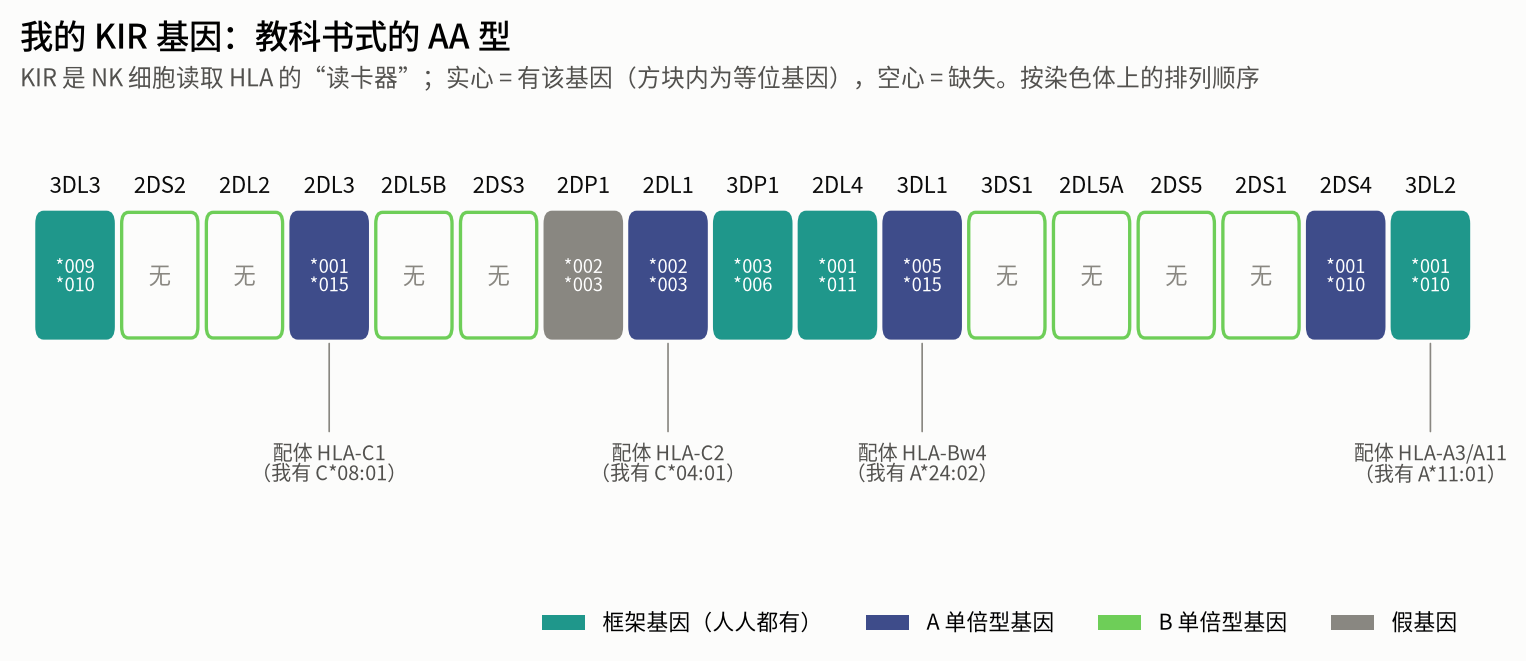
My KIR gene content (T1K typing): genotype AA, none of the activating genes specific to B haplotypes.
| Gene | Result |
|---|---|
| KIR2DL1 | KIR2DL1*003 / KIR2DL1*002 |
| KIR2DL2 | absent |
| KIR2DL3 | KIR2DL3*015 / KIR2DL3*001 |
| KIR2DL4 | KIR2DL4*011 / KIR2DL4*001 |
| KIR2DL5A | absent |
| KIR2DL5B | absent |
| KIR2DP1 | KIR2DP1*003 / KIR2DP1*002 |
| KIR2DS1 | absent |
| KIR2DS2 | absent |
| KIR2DS3 | absent |
| KIR2DS4 | KIR2DS4*001 / KIR2DS4*010 |
| KIR2DS5 | absent |
| KIR3DL1 | KIR3DL1*005 / KIR3DL1*015 |
| KIR3DL2 | KIR3DL2*010 / KIR3DL2*001 |
| KIR3DL3 | KIR3DL3*010 / KIR3DL3*009 |
| KIR3DP1 | KIR3DP1*006 / KIR3DP1*003 |
| KIR3DS1 | absent |
- I am genotype AA: I carry only the A-haplotype genes (2DL1, 2DL3, 2DS4, 3DL1) and none of the activating genes specific to B haplotypes (2DS1, 2DS2, 2DS3, 2DS5, 3DS1). About half of Han Chinese are AA88.
- The readers and the ID cards match well: the inhibitory receptors KIR2DL1, KIR2DL3 and KIR3DL1 all have their HLA ligands (C*04:01 is group C2, C*08:01 group C1, and A*24:02 carries the Bw4 epitope), and I also have HLA-A*11, the ligand of KIR3DL2.
- I carry none of the drug-related HLA risk types (B*15:02 for carbamazepine89, B*58:01 for allopurinol90, and others).
Method: T1K36 (kir-wgs preset) with an index built on the spot from IPD-KIR91; HLA also with T1K (IPD-IMGT/HLA 3.65.0). KIR is one of the hardest regions of the genome to type, so allele-level results are for reference only.
"Non-human" DNA in my blood#
Of my 590 million reads, 1.07 million (0.18%) do not align to the human reference. Most of them have a GC content of 50–80%, while human DNA averages about 41%, so they mostly look bacterial rather than human. The Selfish Gene puts forward a fascinating idea: genes are the protagonists, and we are merely the vehicles they use to replicate92. Seen from the gene's point of view, a lot of behaviour starts to make sense: parents sacrificing themselves for their children, worker bees that never reproduce yet labour for the queen, cordyceps fungi changing the behaviour of the ants they infect. So genes of many other species would "like" to get into the human genome and spread, and viruses are best placed to do it. I classified these "non-human" reads one by one:
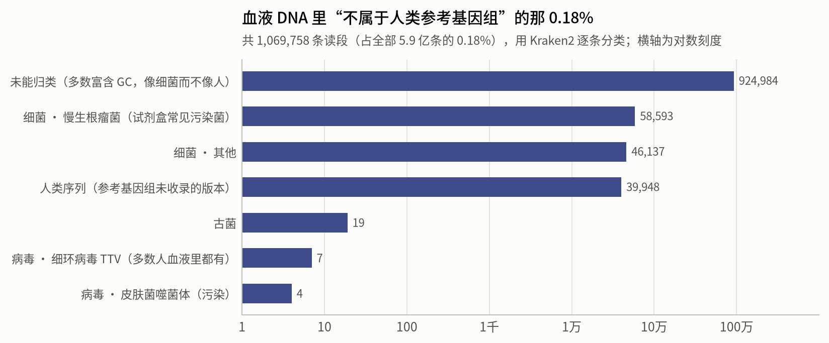
Classification of the 1,069,758 reads that do not align to the human reference (Kraken2):
| Category | Reads |
|---|---|
| Unclassified (mostly GC-rich, bacterial rather than human) | 924,984 |
| Bacteria · Bradyrhizobium (common kit contaminant) | 58,593 |
| Bacteria · other | 46,137 |
| Human (sequence missing from the reference) | 39,948 |
| Archaea | 19 |
| Virus · torque teno virus (in most people's blood) | 7 |
| Virus · phages of skin bacteria (contamination) | 4 |
- More than half of the bacterial reads are Bradyrhizobium, the most common contaminant of sequencing kits and ultrapure water, not something living in me93.
- Only two kinds of virus were found: 7 reads of torque teno virus (TTV), which is in the blood of more than 90% of people and considered essentially harmless94; and 4 reads of phages of skin bacteria (contamination).
- No hepatitis B virus, HPV, HIV and so on; and no inherited chromosomally integrated HHV-6 (about 1% of people are born with a copy of the HHV-6 genome in every cell, which shows up as tens of thousands of reads95).
- At first there seemed to be 51 Epstein–Barr virus reads, but checking each one showed they were all short fragments of human reads mis-aligned; there is no evidence of EBV.
Method: unaligned reads plus reads originally aligned to the EBV decoy sequence, classified with Kraken237 2.17.2 and the standard-8GB database (June 2026). Blood DNA reveals only viruses at fairly high load, so "not detected" does not mean "not infected".
7. Genes whose copy number varies#
Textbooks say every gene comes in two copies, but for some genes people naturally differ: some have more, some fewer, some none at all. Click the buttons above the chart to switch genes; hold Ctrl and scroll to zoom:
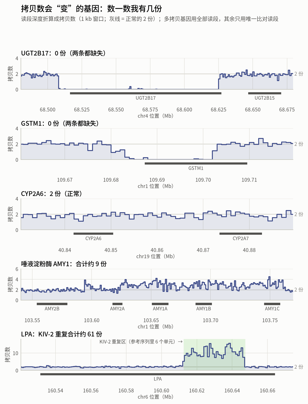
Copy-number-variable genes (estimated from read depth, about ±10%):
| Gene | My copies |
|---|---|
| UGT2B17 | 0.0 |
| GSTM1 | 0.7 |
| CYP2A6 | 1.7 |
| AMY1 | 9.3 |
| C4 | 4.9 |
| RHD | 1.8 |
| Gene | My copies | What it means |
|---|---|---|
| UGT2B17 | 0 (deleted on both) | Very common in East Asians. The enzyme metabolises hormones such as testosterone and some drugs; it also lowers the urinary testosterone/epitestosterone ratio used in doping tests96. |
| GSTM1 | 0 (deleted on both) | True of about half of East Asians. It is a detoxification enzyme, and the deletion is weakly associated with some smoking-related risks. |
| AMY1 (salivary amylase) | about 9 | Ranges from 2 to 17 in the population; populations eating starch-rich diets have more on average97. |
| LPA KIV-2 repeat | about 61 (both copies together) | More repeats mean larger lipoprotein(a) particles and usually lower blood levels. Lp(a) is an independent cardiovascular risk factor, mainly determined by genes; my high repeat count suggests my Lp(a) is probably not high, but it is best measured directly with a blood test (once in a lifetime is enough)98. |
| CYP2A6 | 2 | No whole-gene deletion, which is common in East Asians and slows nicotine metabolism. |
| C4 complement | about 5 | Most people have 499. |
Method: copy number = 2 × mean depth of the region ÷ mean autosomal depth (same filters). For multi-copy or highly homologous genes (AMY1, C4, LPA KIV-2) all reads were used and the copies in the reference were summed; for single-copy genes only uniquely aligned reads. Depth-based absolute values carry an error of about ±10%.
8. Actionable conditions and drug response#
Some gene sites are commonly screened:
- In the 84 genes ACMG recommends for early intervention25 (hereditary cancers, cardiomyopathies and arrhythmias, familial hypercholesterolemia, Marfan syndrome and others), no pathogenic or likely pathogenic variant was found. Not finding one does not mean zero risk, but at least there is no known high-risk variant.
- APOE is ε3/ε3, the most common type, with average population risk for Alzheimer's disease.
Recessive carrier results contain more private information, so I will not go into them here.
Genes that affect drugs#
Pharmacogenomics is the most useful part of whole-genome sequencing. Following the CPIC/DPWG guidelines39,100, I typed genes with PharmCAT38, and CYP2D6 separately with Cyrius101:
| Gene | My phenotype | Drugs affected | What it means in practice |
|---|---|---|---|
| CYP2C19 | Intermediate metabolizer (*1/*2) | Clopidogrel, PPIs, some antidepressants | Clopidogrel may work less well for antiplatelet therapy after a stent or stroke |
| CYP2D6 | Intermediate metabolizer (*10/*36+*10) | Codeine, tramadol, tamoxifen | These painkillers may be weaker for me |
| VKORC1 | Sensitive (−1639 A/A) | Warfarin | Needs a lower dose than Western standards, as most East Asians do |
| ABCG2 | Reduced function (Q141K heterozygous) | Rosuvastatin, allopurinol | Higher rosuvastatin blood levels; start with a low dose |
| CYP3A5 | Intermediate metabolizer | Tacrolimus | Starting dose needs adjusting after organ transplantation |
| CYP2B6 | Intermediate metabolizer | Efavirenz, methadone | |
| NAT2 | Rapid acetylator | Isoniazid | Relatively low risk of liver toxicity from this TB drug |
| Others | Normal | DPYD, TPMT, NUDT15, UGT1A1, G6PD, SLCO1B1, CYP2C9 and others | Standard dosing |
9. Polygenic risk scores#
Adding up hundreds or thousands of "small-effect" variants estimates where your "genetic background" for a disease sits in the population. I used scores developed in East Asian or Chinese populations (from the PGS Catalog40, computed with PLINK 241) and compared myself with 585 East Asians from 1000 Genomes:
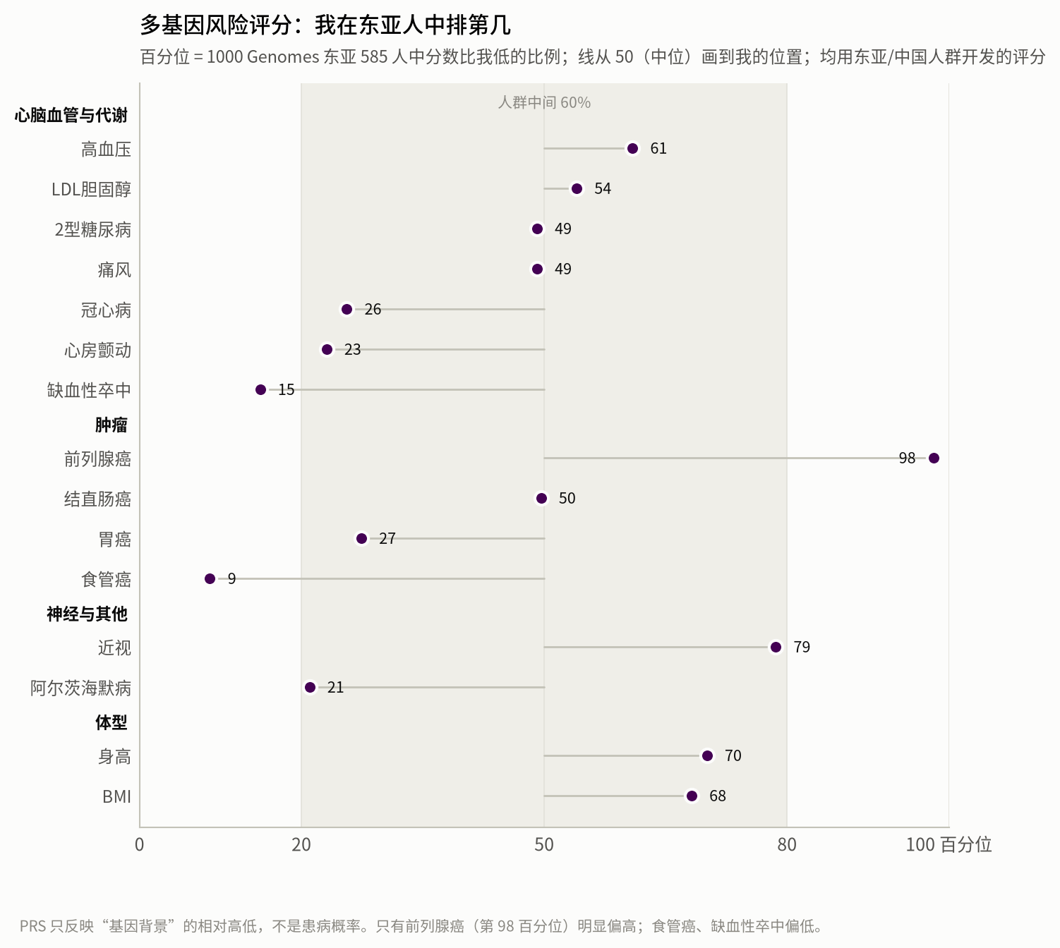
Polygenic risk score percentiles among 585 East Asians in 1000 Genomes (relative position, not the probability of disease):
| Trait | Percentile | PGS | Source |
|---|---|---|---|
| Prostate cancer | 98 | PGS018563 | TPMI 2025 PRS-CS (Taiwanese Han) |
| Myopia | 79 | PGS019957 | Lin 2024 prs149_myopia |
| Height | 70 | PGS002803 | Yengo 2022 GIANT EAS weights |
| BMI | 68 | PGS012556 | Xu 2026 BMI_EAS_MIXPRSplus |
| Hypertension | 61 | PGS005144 | Jung 2025 PRS-CS EAS |
| LDL cholesterol | 54 | PGS004643 | Zhang 2024 LDL_EAS_ldpred2 |
| Colorectal cancer | 50 | PGS002742 | Ping 2022 PRS115_EAS |
| Type 2 diabetes | 49 | PGS005365 | Huerta-Chagoya 2025 DPRISM trained for EAS |
| Gout | 49 | PGS018825 | TPMI 2025 PRS-CS (Taiwanese Han) |
| Gastric cancer | 27 | PGS005161 | Zhu 2025 PRS-GC (Chinese) |
| Coronary artery disease | 26 | PGS004941 | China Kadoorie Biobank 2024 CAD_MetaPRS (developed and validated in Chinese) |
| Atrial fibrillation | 23 | PGS012536 | Haydarlou 2026 Mult-t-EAS |
| Alzheimer's disease | 21 | PGS004589 | Jung 2022 PRS80_trans (APOE reported separately) |
| Ischemic stroke | 15 | PGS002725 | GIGASTROKE 2022 iPGS_EAS |
| Esophageal cancer | 9 | PGS018478 | TPMI 2025 PRS-CS (Taiwanese Han) |
Only prostate cancer (98th percentile) is clearly high; esophageal cancer and ischemic stroke are low, and the rest are within the bulk of the population. A polygenic score reflects relative position, not the probability of disease: the baseline incidence of prostate cancer is not high, so the 98th percentile means it is worth doing PSA screening on schedule when the time comes, not that I "will get it".
10. Repeat expansions in neuromuscular disease#
Neuromuscular disease is my specialty, so I paid special attention to repeat-expansion disorders. Repeat counts were estimated from the reads with ExpansionHunter42. None of the 51 known pathogenic repeat loci102 (myotonic dystrophy types 1 and 2, oculopharyngeal muscular dystrophy, neuronal intranuclear inclusion disease, OPDM, CANVAS, SCA27B, Huntington's disease, several spinocerebellar ataxias and others) shows a pathogenic expansion.
The only "abnormal" result is RFC1: one allele has about 72 repeats, above the normal upper limit. But looking directly at reads that span the whole repeat, the expanded unit is AAAGG, a benign polymorphism common in the population, not the AAGGG that causes CANVAS103. No clinical significance.
11. A WGS self-analysis skill#
WGS can tell you a great deal: the past of your genes (where your ancestors came from), their present (drug-metabolism variants), and a prediction of their future (cancer risk). I packaged the whole analysis pipeline above into a skill: give this link to an AI and let it generate your own genome report.
Tools and data: Parabricks 4.7 (fq2bam, DeepVariant)13,16, GLnexus17, samtools / bcftools104, mosdepth5, Picard6, VEP 11618 + SpliceAI23, ExpansionHunter42, T1K36, Cyrius101, PharmCAT38, PLINK 241, AADR v66.p128, ADMIXTOOLS27, EIGENSOFT26, Beagle 5.529, RFMix v230, hmmix31, bcftools roh32, Yleaf33, HaploGrep 334, Kraken237, TelSeq35; reference genome GRCh38 no-alt + hs38d112; reference populations 1000 Genomes44,45, HGDP43, SGDP53. Charts made with ECharts105, all in the viridis palette.
References#
- Bentley DR, Balasubramanian S, Swerdlow HP, et al. Accurate whole human genome sequencing using reversible terminator chemistry. Nature. 2008;456(7218):53–59. https://doi.org/10.1038/nature07517
- Illumina. NovaSeq X Series specifications. https://www.illumina.com/systems/sequencing-platforms/novaseq-x-plus/specifications.html
- Illumina. Chemistry and imaging on the NovaSeq X Series instruments. https://knowledge.illumina.com/instrumentation/novaseq-x-x-plus/instrumentation-novaseq-x-x-plus-reference_material-list/000007970
- Ewing B, Green P. Base-Calling of Automated Sequencer Traces Using Phred. II. Error Probabilities. Genome Res. 1998;8(3):186–194. https://doi.org/10.1101/gr.8.3.186
- Pedersen BS, Quinlan AR. Mosdepth: quick coverage calculation for genomes and exomes. Bioinformatics. 2018;34(5):867–868. https://doi.org/10.1093/bioinformatics/btx699
- Broad Institute. Picard toolkit: MarkDuplicates. https://broadinstitute.github.io/picard/
- Zhang F, Flickinger M, Taliun SAG, et al. Ancestry-agnostic estimation of DNA sample contamination from sequence reads. Genome Res. 2020;30(2):185–194. https://doi.org/10.1101/gr.246934.118
- Cock PJA, Fields CJ, Goto N, et al. The Sanger FASTQ file format for sequences with quality scores, and the Solexa/Illumina FASTQ variants. Nucleic Acids Res. 2010;38(6):1767–1771. https://doi.org/10.1093/nar/gkp1137
- Li H, Handsaker B, Wysoker A, et al. The Sequence Alignment/Map format and SAMtools. Bioinformatics. 2009;25(16):2078–2079. https://doi.org/10.1093/bioinformatics/btp352
- Bonfield JK. CRAM 3.1: advances in the CRAM file format. Bioinformatics. 2022;38(6):1497–1503. https://doi.org/10.1093/bioinformatics/btac010
- Danecek P, Auton A, Abecasis G, et al. The variant call format and VCFtools. Bioinformatics. 2011;27(15):2156–2158. https://doi.org/10.1093/bioinformatics/btr330
- Schneider VA, Graves-Lindsay T, Howe K, et al. Evaluation of GRCh38 and de novo haploid genome assemblies demonstrates the enduring quality of the reference assembly. Genome Res. 2017;27(5):849–864. https://doi.org/10.1101/gr.213611.116
- NVIDIA. Clara Parabricks 4.7 documentation: fq2bam, DeepVariant. https://docs.nvidia.com/clara/parabricks/
- Li H, Durbin R. Fast and accurate short read alignment with Burrows–Wheeler transform. Bioinformatics. 2009;25(14):1754–1760. https://doi.org/10.1093/bioinformatics/btp324
- Li H. Aligning sequence reads, clone sequences and assembly contigs with BWA-MEM. arXiv. 2013:1303.3997. https://arxiv.org/abs/1303.3997
- Poplin R, Chang PC, Alexander D, et al. A universal SNP and small-indel variant caller using deep neural networks. Nat Biotechnol. 2018;36(10):983–987. https://doi.org/10.1038/nbt.4235
- Yun T, Li H, Chang PC, et al. Accurate, scalable cohort variant calls using DeepVariant and GLnexus. Bioinformatics. 2021;36(24):5582–5589. https://doi.org/10.1093/bioinformatics/btaa1081
- McLaren W, Gil L, Hunt SE, et al. The Ensembl Variant Effect Predictor. Genome Biol. 2016;17(1):122. https://doi.org/10.1186/s13059-016-0974-4
- Karczewski KJ, Francioli LC, Tiao G, et al. The mutational constraint spectrum quantified from variation in 141,456 humans. Nature. 2020;581(7809):434–443. https://doi.org/10.1038/s41586-020-2308-7
- Landrum MJ, Lee JM, Benson M, et al. ClinVar: improving access to variant interpretations and supporting evidence. Nucleic Acids Res. 2018;46(D1):D1062–D1067. https://doi.org/10.1093/nar/gkx1153
- Ioannidis NM, Rothstein JH, Pejaver V, et al. REVEL: An Ensemble Method for Predicting the Pathogenicity of Rare Missense Variants. Am J Hum Genet. 2016;99(4):877–885. https://doi.org/10.1016/j.ajhg.2016.08.016
- Cheng J, Novati G, Pan J, et al. Accurate proteome-wide missense variant effect prediction with AlphaMissense. Science. 2023;381(6664):eadg7492. https://doi.org/10.1126/science.adg7492
- Jaganathan K, Kyriazopoulou Panagiotopoulou S, McRae JF, et al. Predicting Splicing from Primary Sequence with Deep Learning. Cell. 2019;176(3):535–548.e24. https://doi.org/10.1016/j.cell.2018.12.015
- Richards S, Aziz N, Bale S, et al. Standards and guidelines for the interpretation of sequence variants: a joint consensus recommendation of the American College of Medical Genetics and Genomics and the Association for Molecular Pathology. Genet Med. 2015;17(5):405–424. https://doi.org/10.1038/gim.2015.30
- Lee K, Abul-Husn NS, Amendola LM, et al. ACMG SF v3.3 list for reporting of secondary findings in clinical exome and genome sequencing: A policy statement of the American College of Medical Genetics and Genomics (ACMG). Genet Med. 2025;27(8):101454. https://doi.org/10.1016/j.gim.2025.101454
- Patterson N, Price AL, Reich D. Population Structure and Eigenanalysis. PLoS Genet. 2006;2(12):e190. https://doi.org/10.1371/journal.pgen.0020190
- Patterson N, Moorjani P, Luo Y, et al. Ancient Admixture in Human History. Genetics. 2012;192(3):1065–1093. https://doi.org/10.1534/genetics.112.145037
- Mallick S, Micco A, Mah M, et al. The Allen Ancient DNA Resource (AADR) a curated compendium of ancient human genomes. Sci Data. 2024;11(1):182. https://doi.org/10.1038/s41597-024-03031-7
- Browning BL, Tian X, Zhou Y, et al. Fast two-stage phasing of large-scale sequence data. Am J Hum Genet. 2021;108(10):1880–1890. https://doi.org/10.1016/j.ajhg.2021.08.005
- Maples BK, Gravel S, Kenny EE, et al. RFMix: A Discriminative Modeling Approach for Rapid and Robust Local-Ancestry Inference. Am J Hum Genet. 2013;93(2):278–288. https://doi.org/10.1016/j.ajhg.2013.06.020
- Skov L, Hui R, Shchur V, et al. Detecting archaic introgression using an unadmixed outgroup. PLoS Genet. 2018;14(9):e1007641. https://doi.org/10.1371/journal.pgen.1007641
- Narasimhan V, Danecek P, Scally A, et al. BCFtools/RoH: a hidden Markov model approach for detecting autozygosity from next-generation sequencing data. Bioinformatics. 2016;32(11):1749–1751. https://doi.org/10.1093/bioinformatics/btw044
- Ralf A, Montiel González D, Zhong K, et al. Yleaf: Software for Human Y-Chromosomal Haplogroup Inference from Next-Generation Sequencing Data. Mol Biol Evol. 2018;35(5):1291–1294. https://doi.org/10.1093/molbev/msy032
- Schönherr S, Weissensteiner H, Kronenberg F, et al. Haplogrep 3 - an interactive haplogroup classification and analysis platform. Nucleic Acids Res. 2023;51(W1):W263–W268. https://doi.org/10.1093/nar/gkad284
- Ding Z, Mangino M, Aviv A, et al. Estimating telomere length from whole genome sequence data. Nucleic Acids Res. 2014;42(9):e75. https://doi.org/10.1093/nar/gku181
- Song L, Bai G, Liu XS, et al. Efficient and accurate KIR and HLA genotyping with massively parallel sequencing data. Genome Res. 2023;33(6):923–931. https://doi.org/10.1101/gr.277585.122
- Wood DE, Lu J, Langmead B. Improved metagenomic analysis with Kraken 2. Genome Biol. 2019;20(1):257. https://doi.org/10.1186/s13059-019-1891-0
- Sangkuhl K, Whirl‐Carrillo M, Whaley RM, et al. Pharmacogenomics Clinical Annotation Tool (PharmCAT). Clin Pharmacol Ther. 2020;107(1):203–210. https://doi.org/10.1002/cpt.1568
- Relling MV, Klein TE. CPIC: Clinical Pharmacogenetics Implementation Consortium of the Pharmacogenomics Research Network. Clin Pharmacol Ther. 2011;89(3):464–467. https://doi.org/10.1038/clpt.2010.279
- Lambert SA, Gil L, Jupp S, et al. The Polygenic Score Catalog as an open database for reproducibility and systematic evaluation. Nat Genet. 2021;53(4):420–425. https://doi.org/10.1038/s41588-021-00783-5
- Chang CC, Chow CC, Tellier LC, et al. Second-generation PLINK: rising to the challenge of larger and richer datasets. GigaScience. 2015;4:7. https://doi.org/10.1186/s13742-015-0047-8
- Dolzhenko E, Deshpande V, Schlesinger F, et al. ExpansionHunter: a sequence-graph-based tool to analyze variation in short tandem repeat regions. Bioinformatics. 2019;35(22):4754–4756. https://doi.org/10.1093/bioinformatics/btz431
- Bergström A, McCarthy SA, Hui R, et al. Insights into human genetic variation and population history from 929 diverse genomes. Science. 2020;367(6484):eaay5012. https://doi.org/10.1126/science.aay5012
- The 1000 Genomes Project Consortium. A global reference for human genetic variation. Nature. 2015;526(7571):68–74. https://doi.org/10.1038/nature15393
- Byrska-Bishop M, Evani US, Zhao X, et al. High-coverage whole-genome sequencing of the expanded 1000 Genomes Project cohort including 602 trios. Cell. 2022;185(18):3426–3440.e19. https://doi.org/10.1016/j.cell.2022.08.004
- Ning C, Li T, Wang K, et al. Ancient genomes from northern China suggest links between subsistence changes and human migration. Nat Commun. 2020;11(1):2700. https://doi.org/10.1038/s41467-020-16557-2
- Wang CC, Yeh HY, Popov AN, et al. Genomic insights into the formation of human populations in East Asia. Nature. 2021;591(7850):413–419. https://doi.org/10.1038/s41586-021-03336-2
- Fang H, Liang F, Ma H, et al. Dynamic history of the Central Plain and Haidai region inferred from Late Neolithic to Iron Age ancient human genomes. Cell Rep. 2025;44(2):115262. https://doi.org/10.1016/j.celrep.2025.115262
- Jeong C, Wang K, Wilkin S, et al. A Dynamic 6,000-Year Genetic History of Eurasia’s Eastern Steppe. Cell. 2020;183(4):890–904.e29. https://doi.org/10.1016/j.cell.2020.10.015
- Haak W, Lazaridis I, Patterson N, et al. Massive migration from the steppe was a source for Indo-European languages in Europe. Nature. 2015;522(7555):207–211. https://doi.org/10.1038/nature14317
- Harney É, Patterson N, Reich D, et al. Assessing the performance of qpAdm: a statistical tool for studying population admixture. Genetics. 2021;217(4):iyaa045. https://doi.org/10.1093/genetics/iyaa045
- Yang MA, Fan X, Sun B, et al. Ancient DNA indicates human population shifts and admixture in northern and southern China. Science. 2020;369(6501):282–288. https://doi.org/10.1126/science.aba0909
- Mallick S, Li H, Lipson M, et al. The Simons Genome Diversity Project: 300 genomes from 142 diverse populations. Nature. 2016;538(7624):201–206. https://doi.org/10.1038/nature18964
- Fu Q, Li H, Moorjani P, et al. Genome sequence of a 45,000-year-old modern human from western Siberia. Nature. 2014;514(7523):445–449. https://doi.org/10.1038/nature13810
- Seguin-Orlando A, Korneliussen TS, Sikora M, et al. Genomic structure in Europeans dating back at least 36,200 years. Science. 2014;346(6213):1113–1118. https://doi.org/10.1126/science.aaa0114
- Mondal M, Casals F, Xu T, et al. Genomic analysis of Andamanese provides insights into ancient human migration into Asia and adaptation. Nat Genet. 2016;48(9):1066–1070. https://doi.org/10.1038/ng.3621
- Yang MA, Gao X, Theunert C, et al. 40,000-Year-Old Individual from Asia Provides Insight into Early Population Structure in Eurasia. Curr Biol. 2017;27(20):3202–3208.e9. https://doi.org/10.1016/j.cub.2017.09.030
- Lazaridis I, Nadel D, Rollefson G, et al. Genomic insights into the origin of farming in the ancient Near East. Nature. 2016;536(7617):419–424. https://doi.org/10.1038/nature19310
- Cooke NP, Mattiangeli V, Cassidy LM, et al. Ancient genomics reveals tripartite origins of Japanese populations. Sci Adv. 2021;7(38):eabh2419. https://doi.org/10.1126/sciadv.abh2419
- Mao X, Zhang H, Qiao S, et al. The deep population history of northern East Asia from the Late Pleistocene to the Holocene. Cell. 2021;184(12):3256–3266.e13. https://doi.org/10.1016/j.cell.2021.04.040
- Sikora M, Pitulko VV, Sousa VC, et al. The population history of northeastern Siberia since the Pleistocene. Nature. 2019;570(7760):182–188. https://doi.org/10.1038/s41586-019-1279-z
- Wang T, Wang W, Xie G, et al. Human population history at the crossroads of East and Southeast Asia since 11,000 years ago. Cell. 2021;184(14):3829–3841.e21. https://doi.org/10.1016/j.cell.2021.05.018
- Liu J, Liu Y, Zhao Y, et al. East Asian Gene flow bridged by northern coastal populations over past 6000 years. Nat Commun. 2025;16(1):1322. https://doi.org/10.1038/s41467-025-56555-w
- YFull. YTree v14.01: O-MF1484. https://www.yfull.com/tree/O-MF1484/
- FamilyTreeDNA. Y-DNA Haplotree. https://discover.familytreedna.com/
- Yang T, He J, Li C, et al. Ancient DNA reveals the population interactions and a Neolithic patrilineal community in Northern Yangtze Region. Nat Commun. 2025;16(1):8728. https://doi.org/10.1038/s41467-025-63743-1
- Wang T, Yang MA, Zhu Z, et al. Prehistoric genomes from Yunnan reveal ancestry related to Tibetans and Austroasiatic speakers. Science. 2025;388(6750):eadq9792. https://doi.org/10.1126/science.adq9792
- Maróti Z, Neparáczki E, Schütz O, et al. The genetic origin of Huns, Avars, and conquering Hungarians. Curr Biol. 2022;32(13):2858–2870.e7. https://doi.org/10.1016/j.cub.2022.04.093
- Gnecchi-Ruscone GA, Rácz Z, Samu L, et al. Network of large pedigrees reveals social practices of Avar communities. Nature. 2024;629(8011):376–383. https://doi.org/10.1038/s41586-024-07312-4
- International Society of Genetic Genealogy. ISOGG Y-DNA Haplogroup Tree. https://isogg.org/tree/
- Sankararaman S, Mallick S, Patterson N, et al. The Combined Landscape of Denisovan and Neanderthal Ancestry in Present-Day Humans. Curr Biol. 2016;26(9):1241–1247. https://doi.org/10.1016/j.cub.2016.03.037
- Prüfer K, de Filippo C, Grote S, et al. A high-coverage Neandertal genome from Vindija Cave in Croatia. Science. 2017;358(6363):655–658. https://doi.org/10.1126/science.aao1887
- The SIGMA Type 2 Diabetes Consortium. Sequence variants in SLC16A11 are a common risk factor for type 2 diabetes in Mexico. Nature. 2014;506(7486):97–101. https://doi.org/10.1038/nature12828
- Abi-Rached L, Jobin MJ, Kulkarni S, et al. The Shaping of Modern Human Immune Systems by Multiregional Admixture with Archaic Humans. Science. 2011;334(6052):89–94. https://doi.org/10.1126/science.1209202
- Ding Q, Hu Y, Xu S, et al. Neanderthal Introgression at Chromosome 3p21.31 Was Under Positive Natural Selection in East Asians. Mol Biol Evol. 2014;31(3):683–695. https://doi.org/10.1093/molbev/mst260
- Vernot B, Akey JM. Resurrecting Surviving Neandertal Lineages from Modern Human Genomes. Science. 2014;343(6174):1017–1021. https://doi.org/10.1126/science.1245938
- Sankararaman S, Mallick S, Dannemann M, et al. The genomic landscape of Neanderthal ancestry in present-day humans. Nature. 2014;507(7492):354–357. https://doi.org/10.1038/nature12961
- Prüfer K, Racimo F, Patterson N, et al. The complete genome sequence of a Neanderthal from the Altai Mountains. Nature. 2014;505(7481):43–49. https://doi.org/10.1038/nature12886
- Mafessoni F, Grote S, de Filippo C, et al. A high-coverage Neandertal genome from Chagyrskaya Cave. Proc Natl Acad Sci USA. 2020;117(26):15132–15136. https://doi.org/10.1073/pnas.2004944117
- Meyer M, Kircher M, Gansauge MT, et al. A High-Coverage Genome Sequence from an Archaic Denisovan Individual. Science. 2012;338(6104):222–226. https://doi.org/10.1126/science.1224344
- Ceballos FC, Joshi PK, Clark DW, et al. Runs of homozygosity: windows into population history and trait architecture. Nat Rev Genet. 2018;19(4):220–234. https://doi.org/10.1038/nrg.2017.109
- Mengel-From J, Thinggaard M, Dalgård C, et al. Mitochondrial DNA copy number in peripheral blood cells declines with age and is associated with general health among elderly. Hum Genet. 2014;133(9):1149–1159. https://doi.org/10.1007/s00439-014-1458-9
- Jaiswal S, Fontanillas P, Flannick J, et al. Age-Related Clonal Hematopoiesis Associated with Adverse Outcomes. N Engl J Med. 2014;371(26):2488–2498. https://doi.org/10.1056/NEJMoa1408617
- Genovese G, Kähler AK, Handsaker RE, et al. Clonal Hematopoiesis and Blood-Cancer Risk Inferred from Blood DNA Sequence. N Engl J Med. 2014;371(26):2477–2487. https://doi.org/10.1056/NEJMoa1409405
- Forsberg LA, Rasi C, Malmqvist N, et al. Mosaic loss of chromosome Y in peripheral blood is associated with shorter survival and higher risk of cancer. Nat Genet. 2014;46(6):624–628. https://doi.org/10.1038/ng.2966
- ISBT Working Party on Red Cell Immunogenetics and Blood Group Terminology. Blood group allele tables. https://www.isbtweb.org/isbt-working-parties/rcibgt.html
- Barker DJ, Maccari G, Georgiou X, et al. The IPD-IMGT/HLA Database. Nucleic Acids Res. 2023;51(D1):D1053–D1060. https://doi.org/10.1093/nar/gkac1011
- Gonzalez-Galarza FF, McCabe A, Santos EJMD, et al. Allele frequency net database (AFND) 2020 update: gold-standard data classification, open access genotype data and new query tools. Nucleic Acids Res. 2020;48(D1):D783–D788. https://doi.org/10.1093/nar/gkz1029
- Chung WH, Hung SI, Hong HS, et al. A marker for Stevens–Johnson syndrome. Nature. 2004;428(6982):486. https://doi.org/10.1038/428486a
- Hung SI, Chung WH, Liou LB, et al. HLA-B*5801 allele as a genetic marker for severe cutaneous adverse reactions caused by allopurinol. Proc Natl Acad Sci USA. 2005;102(11):4134–4139. https://doi.org/10.1073/pnas.0409500102
- Robinson J, Halliwell JA, McWilliam H, et al. IPD—the Immuno Polymorphism Database. Nucleic Acids Res. 2013;41(D1):D1234–D1240. https://doi.org/10.1093/nar/gks1140
- Dawkins R. The Selfish Gene. Oxford: Oxford University Press; 1976.
- Salter SJ, Cox MJ, Turek EM, et al. Reagent and laboratory contamination can critically impact sequence-based microbiome analyses. BMC Biol. 2014;12(1):87. https://doi.org/10.1186/s12915-014-0087-z
- Spandole S, Cimponeriu D, Berca LM, et al. Human anelloviruses: an update of molecular, epidemiological and clinical aspects. Arch Virol. 2015;160(4):893–908. https://doi.org/10.1007/s00705-015-2363-9
- Pellett PE, Ablashi DV, Ambros PF, et al. Chromosomally integrated human herpesvirus 6: questions and answers. Rev Med Virol. 2012;22(3):144–155. https://doi.org/10.1002/rmv.715
- Schulze JJ, Lundmark J, Garle M, et al. Doping Test Results Dependent on Genotype of Uridine Diphospho-Glucuronosyl Transferase 2B17, the Major Enzyme for Testosterone Glucuronidation. J Clin Endocrinol Metab. 2008;93(7):2500–2506. https://doi.org/10.1210/jc.2008-0218
- Perry GH, Dominy NJ, Claw KG, et al. Diet and the evolution of human amylase gene copy number variation. Nat Genet. 2007;39(10):1256–1260. https://doi.org/10.1038/ng2123
- Kronenberg F, Mora S, Stroes ESG, et al. Lipoprotein(a) in atherosclerotic cardiovascular disease and aortic stenosis: a European Atherosclerosis Society consensus statement. Eur Heart J. 2022;43(39):3925–3946. https://doi.org/10.1093/eurheartj/ehac361
- Sekar A, Bialas AR, de Rivera H, et al. Schizophrenia risk from complex variation of complement component 4. Nature. 2016;530(7589):177–183. https://doi.org/10.1038/nature16549
- Swen JJ, Nijenhuis M, de Boer A, et al. Pharmacogenetics: From Bench to Byte—An Update of Guidelines. Clin Pharmacol Ther. 2011;89(5):662–673. https://doi.org/10.1038/clpt.2011.34
- Chen X, Shen F, Gonzaludo N, et al. Cyrius: accurate CYP2D6 genotyping using whole-genome sequencing data. Pharmacogenomics J. 2021;21(2):251–261. https://doi.org/10.1038/s41397-020-00205-5
- Clinical Genomics Stockholm. Stranger: annotation of repeat expansions. https://github.com/Clinical-Genomics/stranger
- Cortese A, Simone R, Sullivan R, et al. Biallelic expansion of an intronic repeat in RFC1 is a common cause of late-onset ataxia. Nat Genet. 2019;51(4):649–658. https://doi.org/10.1038/s41588-019-0372-4
- Danecek P, Bonfield JK, Liddle J, et al. Twelve years of SAMtools and BCFtools. GigaScience. 2021;10(2):giab008. https://doi.org/10.1093/gigascience/giab008
- Li D, Mei H, Shen Y, et al. ECharts: A declarative framework for rapid construction of web-based visualization. Vis Inform. 2018;2(2):136–146. https://doi.org/10.1016/j.visinf.2018.04.011